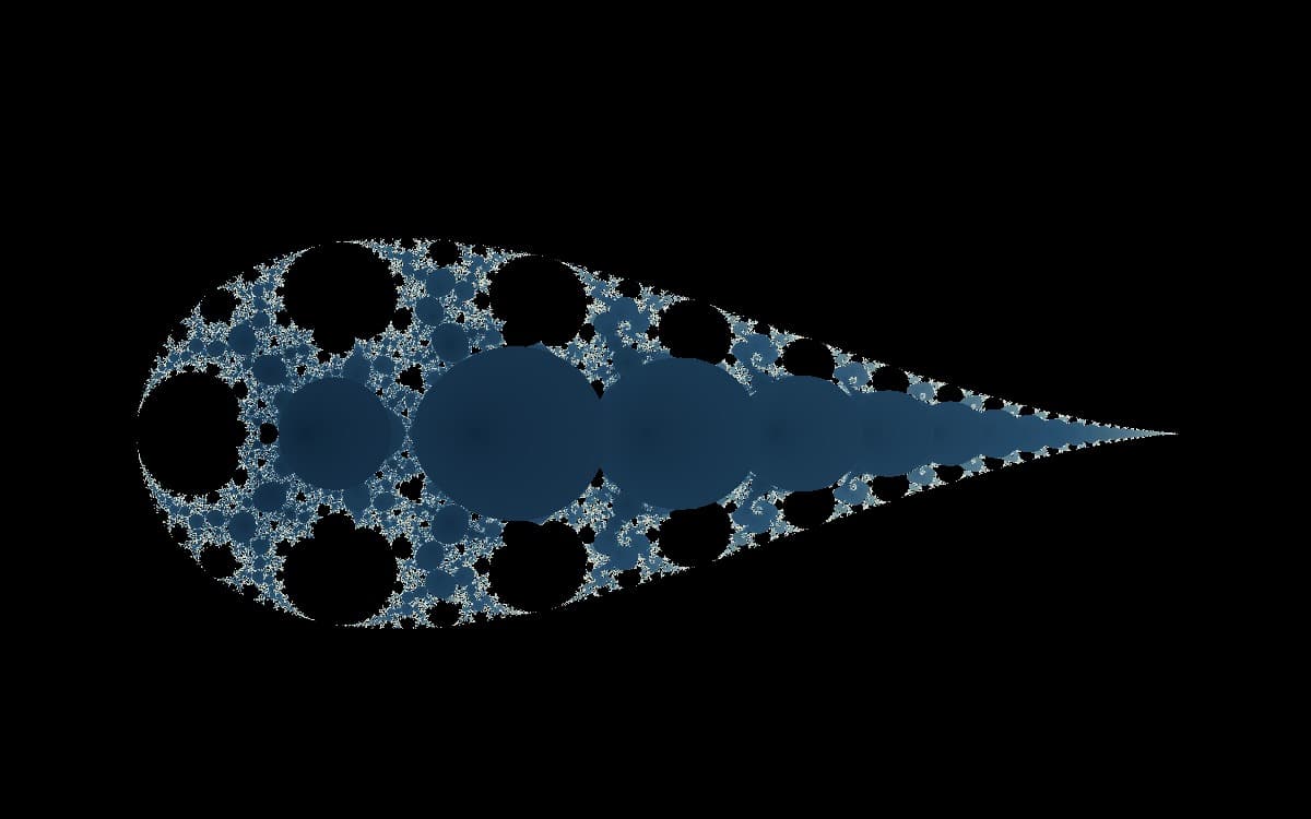
FractalPark
MagnetDifficile

Magnet Type 2

Une application rationnelle au carré avec z² dans le quotient, donnant au terrain du Type 1 une forme plus escarpée et plus plissée.

Ouvrir dans l'Explorateur
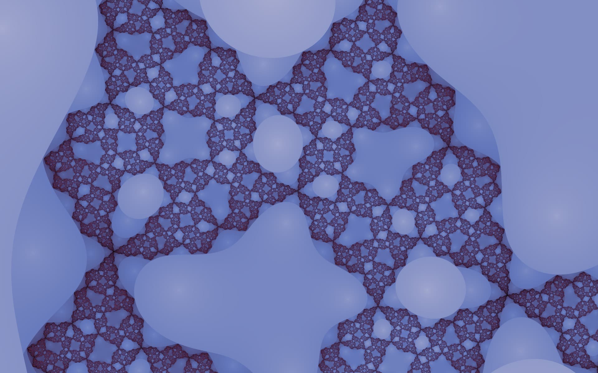
Vue de Julia de Magnet Type 2 à symétrie de croix, avec quatre secteurs répétés d'anneaux, de chaînes de perles et de lobes
Le Magnet Type 2 de FractalPark à c = −0.56 + 0.11i : symétrie de croix d'ordre quatre, anneaux en couches et chaînes de perles, avec des crêtes partant des deux pôles jumeaux.

Vue d'ensemble

Magnet Type 2 itère ((z² + c) / (z² − c))². Il conserve le quotient au carré du Type 1, mais z est déjà au carré dans le numérateur comme dans le dénominateur. Élever ce rapport au carré donne une application rationnelle de degré quatre, soit deux fois le degré du Type 1.

Le degré supplémentaire se voit à deux endroits. Le dénominateur z² − c s'annule en deux valeurs racine carrée de c, et non une seule, ce qui donne deux pôles. La mise au carré répétée aiguise aussi le pli angulaire en symétrie de croix. Avec plus de pôles et plus de rotations, le Type 2 devient plus dense et plus anguleux.

Le mécanisme de la famille aimant demeure. Une orbite passant près d'un pôle est projetée vers une grande valeur, puis se replie vers 1 à l'étape suivante. Elle ne va pas à l'infini : sur la sphère de Riemann, elle est envoyée vers 1. Les bassins se rassemblent à travers le plan, tandis que les préimages du pôle assemblent la frontière fractale entre eux.

Les mathématiques

Type 2 rational iteration

z(n+1) = ((z(n)^2 + c) / (z(n)^2 - c))^2

Each step computes (z² + c) / (z² − c), then squares it. The numerator is zero when z² = −c; the denominator is zero when z² = c. After squaring, every zero and pole is double, leaving the map with two double zeros and two double poles on the Riemann sphere. Its rational degree is four.

As |z| grows, (z² + c) / (z² − c) approaches 1, so the next value lands near 1 no matter how large z becomes. Only a close pass by one of the two poles produces a large value. FractalPark treats |z| above 16 as escaped, so a coloured “fast escape” region records a close encounter with a pole, not a one-way trip to infinity.

Suppose c = 1. The poles are at z² = 1, i.e. z = 1 and z = −1. Choose z₀ = 0.98, very close to the pole at 1. Then (z₀² + c) / (z₀² − c) ≈ (0.9604 + 1) / (0.9604 − 1) = 1.9604 / (−0.0396) ≈ −49.5, and squaring gives z₁ ≈ 2450. The large value then folds back: on the next step, with |z₁| large, the ratio tends to 1 and z₂ lands near 1. The shader colours the pixel according to how quickly the orbit returns near 1 after its pole encounter.

Histoire

In 1986, Heinz-Otto Peitgen and Peter H. Richter brought magnet fractals into the literature in *The Beauty of Fractals: Images of Complex Dynamical Systems*. Their chapter “Magnetism and Complex Boundaries” (pp. 129–138) presented rational maps derived from renormalization transformations in a model of magnetic materials. The boundary between magnetic and non-magnetic phases is fractal; iterating the transformation draws it, giving the images their clustered, field-like structure.

Fractint later included the maps as “magnet1” and “magnet2,” in both Mandelbrot-style and Julia-style views, and the name spread through fractal software. POV-Ray’s documentation still describes its magnet1 and magnet2 patterns as “derived from some magnetic renormalization transformations,” crediting the Fractint help files.

The classic Type 2 formula from that lineage is ((z² + c − 1) / (2z + c − 2))². FractalPark implements a different simplified squared quotient, ((z² + c) / (z² − c))², under the same name; every render and every mathematical statement on this page refers to the formula as FractalPark actually computes it.

Caractéristiques visuelles

The guide image is a Julia-mode view at c = −0.56 + 0.11i. Cross-like symmetry holds the frame together: two intersecting folding axes divide the plane into four repeating sectors, each packed with layered rings, bead-like chains, and lobes. Two opposing bright nodes mark the poles, with angular ridges radiating outward.

At the same parameter, Type 2 has finer angular detail and a more articulated basin boundary than Type 1. The warm core and cool exterior emphasise its radial structure, but the geometry comes from the map: the extra degree reorients the basins along the cross axes set by the two poles.

Remix et exemples

Pars du Document canonique

Ouvre le même état de formule approuvé utilisé par ce guide, puis modifie la vue, la colorisation, les transformations ou l'animation dans l'Explorateur interactif.

Questions fréquentes

How does Type 2 differ from Type 1?

Type 2 squares z before forming the quotient, so its numerator and denominator carry z² rather than z. This raises the rational degree from two to four, takes the number of poles from one to two, and strengthens the cross-like angular symmetry. At the same parameter, its images are denser and more folded than Type 1’s.

Where do its poles occur?

Poles occur where the denominator z² − c vanishes: z = √c and z = −√c. Type 1 has one pole at z = c; Type 2 has two, except when c = 0, when the pole at zero is double. Their positions move with c and strongly influence the fractal boundary’s layout.

Références