FractalPark
МагнитСложно

Magnet Type 2

Возведённое в квадрат рациональное отображение с z² внутри отношения, придающее рельефу Type 1 более крутую, более складчатую форму.

Открыть в Обзоре
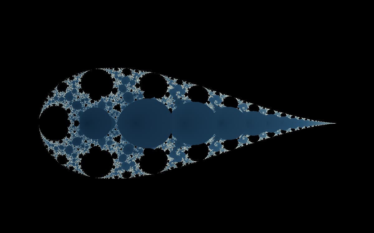
Крестообразно-симметричный вид Жюлиа Magnet Type 2 с четырьмя повторяющимися секторами колец, цепочек-бус и долей
Magnet Type 2 от FractalPark при c = −0.56 + 0.11i: четырёхкратная крестообразная симметрия, слоистые кольца и цепочки-бусы с гребнями, расходящимися от двух полюсов.

Обзор

Magnet Type 2 итерирует ((z² + c) / (z² − c))². Он сохраняет возведённое в квадрат отношение Type 1, но z уже возведено в квадрат и в числителе, и в знаменателе. Возведение этого отношения в квадрат даёт рациональное отображение четвёртой степени — вдвое выше степени Type 1.

Дополнительная степень проявляется в двух местах. Знаменатель z² − c обращается в нуль при двух квадратных корнях из c, а не при одном, — появляются два полюса. Повторное возведение в квадрат также заостряет угловую складку до крестообразной симметрии. С бо́льшим числом полюсов и поворотов Type 2 становится плотнее и угловатее.

Механизм семейства магнитов сохраняется. Орбита, проходящая вблизи полюса, выбрасывается к большому значению, а на следующем шаге складывается обратно к 1. Она не уходит на бесконечность: на сфере Римана она отображается в 1. Бассейны собираются по плоскости, а прообразы полюсов складывают между ними фрактальную границу.

Математика

Type 2 rational iteration

z(n+1) = ((z(n)^2 + c) / (z(n)^2 - c))^2

Each step computes (z² + c) / (z² − c), then squares it. The numerator is zero when z² = −c; the denominator is zero when z² = c. After squaring, every zero and pole is double, leaving the map with two double zeros and two double poles on the Riemann sphere. Its rational degree is four.

As |z| grows, (z² + c) / (z² − c) approaches 1, so the next value lands near 1 no matter how large z becomes. Only a close pass by one of the two poles produces a large value. FractalPark treats |z| above 16 as escaped, so a coloured “fast escape” region records a close encounter with a pole, not a one-way trip to infinity.

Suppose c = 1. The poles are at z² = 1, i.e. z = 1 and z = −1. Choose z₀ = 0.98, very close to the pole at 1. Then (z₀² + c) / (z₀² − c) ≈ (0.9604 + 1) / (0.9604 − 1) = 1.9604 / (−0.0396) ≈ −49.5, and squaring gives z₁ ≈ 2450. The large value then folds back: on the next step, with |z₁| large, the ratio tends to 1 and z₂ lands near 1. The shader colours the pixel according to how quickly the orbit returns near 1 after its pole encounter.
История

In 1986, Heinz-Otto Peitgen and Peter H. Richter brought magnet fractals into the literature in *The Beauty of Fractals: Images of Complex Dynamical Systems*. Their chapter “Magnetism and Complex Boundaries” (pp. 129–138) presented rational maps derived from renormalization transformations in a model of magnetic materials. The boundary between magnetic and non-magnetic phases is fractal; iterating the transformation draws it, giving the images their clustered, field-like structure.

Fractint later included the maps as “magnet1” and “magnet2,” in both Mandelbrot-style and Julia-style views, and the name spread through fractal software. POV-Ray’s documentation still describes its magnet1 and magnet2 patterns as “derived from some magnetic renormalization transformations,” crediting the Fractint help files.

The classic Type 2 formula from that lineage is ((z² + c − 1) / (2z + c − 2))². FractalPark implements a different simplified squared quotient, ((z² + c) / (z² − c))², under the same name; every render and every mathematical statement on this page refers to the formula as FractalPark actually computes it.

Визуальные особенности

The guide image is a Julia-mode view at c = −0.56 + 0.11i. Cross-like symmetry holds the frame together: two intersecting folding axes divide the plane into four repeating sectors, each packed with layered rings, bead-like chains, and lobes. Two opposing bright nodes mark the poles, with angular ridges radiating outward.

At the same parameter, Type 2 has finer angular detail and a more articulated basin boundary than Type 1. The warm core and cool exterior emphasise its radial structure, but the geometry comes from the map: the extra degree reorients the basins along the cross axes set by the two poles.

Ремиксы и примеры

Начните с канонического документа

Откройте то же утверждённое состояние формулы, которое используется в этом руководстве, а затем измените вид, раскраску, трансформации или анимацию в интерактивном Обзоре.

Часто задаваемые вопросы

How does Type 2 differ from Type 1?

Type 2 squares z before forming the quotient, so its numerator and denominator carry z² rather than z. This raises the rational degree from two to four, takes the number of poles from one to two, and strengthens the cross-like angular symmetry. At the same parameter, its images are denser and more folded than Type 1’s.

Where do its poles occur?

Poles occur where the denominator z² − c vanishes: z = √c and z = −√c. Type 1 has one pole at z = c; Type 2 has two, except when c = 0, when the pole at zero is double. Their positions move with c and strongly influence the fractal boundary’s layout.

Ссылки