FractalPark
MagnetMedium

Magnet Type 1

A squared Möbius quotient with one pole at z = c, gathering the plane into clustered basins and bead-like chains.

Open in Explorer
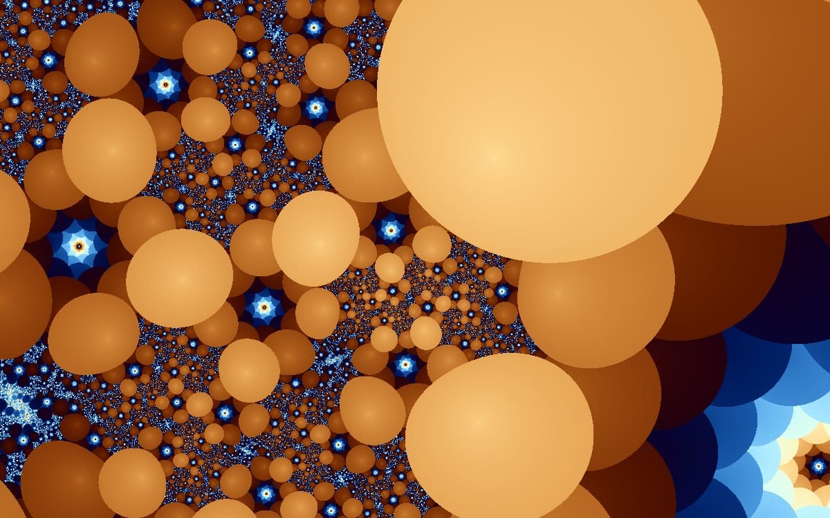
Copper-orange spheres of many sizes clustered over a deep blue field scattered with small blue-and-white star-shaped rosettes
A Julia view of Magnet Type 1: smooth rounded basins gather in clusters, while star-like rosettes crowd their fractal borders.

Overview

Magnet Type 1 starts from ((z + c) / (z − c))². The ratio in parentheses is a Möbius transformation, the simplest non-trivial rational function; squaring it makes a rational map of degree two. Unlike z² + c, this map does not send distant points ever farther away. They turn back toward 1.

The dynamics center on two opposite locations. The quotient is zero at z = −c and has a pole at z = c. An orbit that brushes the pole flies far out, then returns near 1 on its next step. Stable basins spread across the plane; between them is a fractal boundary made from layer after layer of the pole’s preimages.

FractalPark offers a parameter plane, where c moves, and Julia views, where c stays fixed. The guide image is a Julia close-up. Its rounded basins gather in clumps like iron filings around a magnet — hence the family name.

The Mathematics

A Möbius quotient, squared

z(n+1) = ((z(n) + c) / (z(n) - c))^2

Each step forms (z + c) / (z − c), then squares it. The ratio is zero at z = −c and blows up at z = c. Squaring makes −c a double zero and c a double pole, while leaving the map with rational degree two.

Infinity behaves differently here. As |z| grows, (z + c) / (z − c) approaches 1, so the next value lands near 1 however large z becomes. Huge values arise only near z = c. FractalPark treats |z| above 16 as escaped, so a “fast escape” marks a close pass by the pole, not a one-way trip to infinity.

On the Riemann sphere, the pole maps to infinity and infinity maps to 1, so the orbit remains well-defined at the singularity. A numerical renderer cannot divide by zero: when the denominator is exactly zero, the shader substitutes 0, and the next step continues from f(0) = 1. That is a computational safeguard, not another mathematical definition.
History

In 1986, Heinz-Otto Peitgen and Peter H. Richter brought magnet fractals into the literature in *The Beauty of Fractals: Images of Complex Dynamical Systems*. Their chapter “Magnetism and Complex Boundaries” (pp. 129–138) presented rational maps derived from renormalization transformations in a model of magnetic materials. There, the boundary between magnetic and non-magnetic phases is fractal. Iterating the transformation draws that boundary, giving the images their clustered, field-like structure.

Fractint later included the maps as “magnet1” and “magnet2,” in both Mandelbrot-style and Julia-style views; the name was then adopted by other fractal software. POV-Ray’s documentation still calls its magnet1 and magnet2 patterns “derived from some magnetic renormalization transformations,” crediting the Fractint help files.

The classic Type 1 formula from that lineage is ((z² + c − 1) / (2z + c − 2))². FractalPark implements a simplified squared quotient, ((z + c) / (z − c))², under the same name; every render and every mathematical statement on this page refers to the formula as FractalPark actually computes it.

Visual Characteristics

In this Julia-set close-up, large smooth copper-orange spheres gather on the right in clusters of very different sizes. The deep blue at left and below holds smaller spheres and blue-white rosettes, each star-shaped around a faint orange core.

The rounded blobs are basins, where orbits settle. Rosettes and dense grain trace the fractal border between them. This arrangement belongs to this parameter and framing—other c values rearrange it. The warm/cool palette is a colouring choice, not a property of the formula.

Remix and Examples

Start from the canonical Document

Open the same approved formula state used by this guide, then change the view, coloring, transforms, or animation in the interactive Explorer.

Frequently Asked Questions

Why is it called Magnet?

The name comes from a family made widely known by Fractint. Its maps trace back to renormalization calculations for a model of magnetic phase transitions, presented in Heinz-Otto Peitgen and Peter H. Richter’s 1986 book *The Beauty of Fractals*. The squared-quotient formulas form clustered, domain-like basins; their boundaries mark the transition between magnetic and non-magnetic phases.

FractalPark’s Type 1 keeps the name and the squared-quotient shape but uses the simpler ratio ((z + c) / (z − c))². The formula shown on this page is exactly the one the engine computes.

What happens near z = c?

At that point the denominator z − c vanishes. Thus z = c is a pole of the quotient, and a double pole after squaring. Orbits that skim past it leap to very large values, then fold back near 1 a step later.

This behaviour builds the boundary: a growing web of points whose orbits eventually hit the pole. For the rare pixel that lands exactly there, the shader uses a safe value rather than divide by zero, matching the orbit’s continuation on the Riemann sphere.

References