FractalPark
MagnetHard

Magnet Type 2

A squared rational map with z² inside the quotient, giving Type 1’s terrain a steeper, more folded form.

Open in Explorer
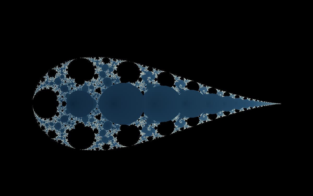
Cross-symmetric Magnet Type 2 Julia view with four repeating sectors of rings, bead chains and lobes
FractalPark’s Magnet Type 2 at c = −0.56 + 0.11i: fourfold cross symmetry, layered rings and bead chains, with ridges running from twin poles.

Overview

Magnet Type 2 iterates ((z² + c) / (z² − c))². It keeps Type 1’s squared quotient, but z is already squared in both numerator and denominator. Squaring that ratio gives a rational map of degree four, twice Type 1’s degree.

The extra degree shows up in two places. The denominator z² − c vanishes at two square-root values of c, not one, giving two poles. Repeated squaring also sharpens the angular fold into cross-like symmetry. With more poles and more turning, Type 2 becomes denser and more angular.

The magnet-family mechanism remains. An orbit passing near a pole is flung to a large value, then folds back toward 1 on the next step. It does not go to infinity: on the Riemann sphere it maps to 1. Basins gather across the plane, while pole preimages assemble the fractal border between them.

The Mathematics

Type 2 rational iteration

z(n+1) = ((z(n)^2 + c) / (z(n)^2 - c))^2

Each step computes (z² + c) / (z² − c), then squares it. The numerator is zero when z² = −c; the denominator is zero when z² = c. After squaring, every zero and pole is double, leaving the map with two double zeros and two double poles on the Riemann sphere. Its rational degree is four.

As |z| grows, (z² + c) / (z² − c) approaches 1, so the next value lands near 1 no matter how large z becomes. Only a close pass by one of the two poles produces a large value. FractalPark treats |z| above 16 as escaped, so a coloured “fast escape” region records a close encounter with a pole, not a one-way trip to infinity.

Suppose c = 1. The poles are at z² = 1, i.e. z = 1 and z = −1. Choose z₀ = 0.98, very close to the pole at 1. Then (z₀² + c) / (z₀² − c) ≈ (0.9604 + 1) / (0.9604 − 1) = 1.9604 / (−0.0396) ≈ −49.5, and squaring gives z₁ ≈ 2450. The large value then folds back: on the next step, with |z₁| large, the ratio tends to 1 and z₂ lands near 1. The shader colours the pixel according to how quickly the orbit returns near 1 after its pole encounter.

History

In 1986, Heinz-Otto Peitgen and Peter H. Richter brought magnet fractals into the literature in *The Beauty of Fractals: Images of Complex Dynamical Systems*. Their chapter “Magnetism and Complex Boundaries” (pp. 129–138) presented rational maps derived from renormalization transformations in a model of magnetic materials. The boundary between magnetic and non-magnetic phases is fractal; iterating the transformation draws it, giving the images their clustered, field-like structure.

Fractint later included the maps as “magnet1” and “magnet2,” in both Mandelbrot-style and Julia-style views, and the name spread through fractal software. POV-Ray’s documentation still describes its magnet1 and magnet2 patterns as “derived from some magnetic renormalization transformations,” crediting the Fractint help files.

The classic Type 2 formula from that lineage is ((z² + c − 1) / (2z + c − 2))². FractalPark implements a different simplified squared quotient, ((z² + c) / (z² − c))², under the same name; every render and every mathematical statement on this page refers to the formula as FractalPark actually computes it.

Visual Characteristics

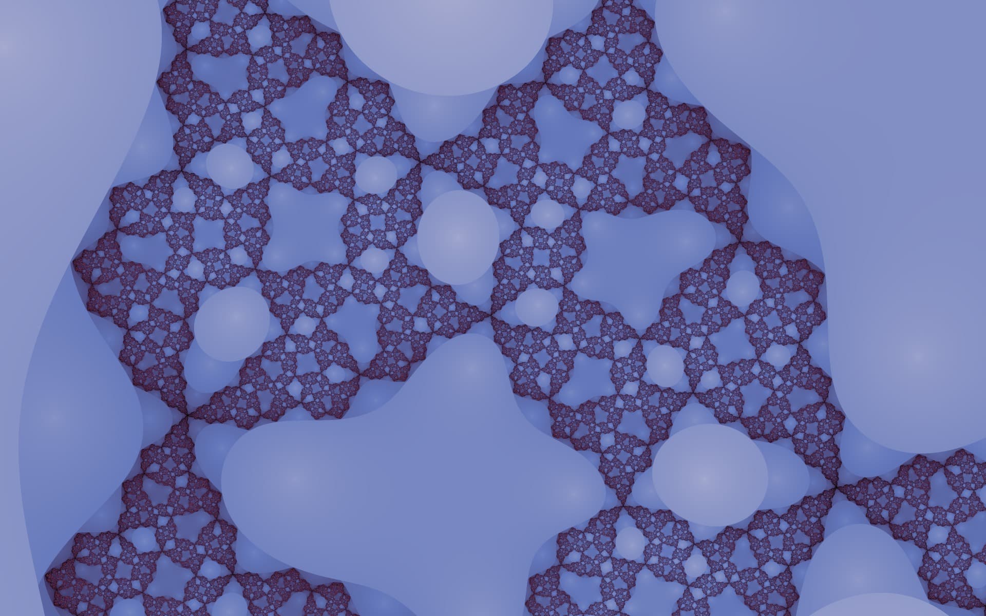
The guide image is a Julia-mode view at c = −0.56 + 0.11i. Cross-like symmetry holds the frame together: two intersecting folding axes divide the plane into four repeating sectors, each packed with layered rings, bead-like chains, and lobes. Two opposing bright nodes mark the poles, with angular ridges radiating outward.

At the same parameter, Type 2 has finer angular detail and a more articulated basin boundary than Type 1. The warm core and cool exterior emphasise its radial structure, but the geometry comes from the map: the extra degree reorients the basins along the cross axes set by the two poles.

Remix and Examples

Start from the canonical Document

Open the same approved formula state used by this guide, then change the view, coloring, transforms, or animation in the interactive Explorer.

Frequently Asked Questions

How does Type 2 differ from Type 1?

Type 2 squares z before forming the quotient, so its numerator and denominator carry z² rather than z. This raises the rational degree from two to four, takes the number of poles from one to two, and strengthens the cross-like angular symmetry. At the same parameter, its images are denser and more folded than Type 1’s.

Where do its poles occur?

Poles occur where the denominator z² − c vanishes: z = √c and z = −√c. Type 1 has one pole at z = c; Type 2 has two, except when c = 0, when the pole at zero is double. Their positions move with c and strongly influence the fractal boundary’s layout.

References